---
title: "From ATE to Uplift Modeling"
format:
html:
toc: true
toc-depth: 3
toc-title: "Contents"
code-fold: false
code-tools: true
theme: cosmo
highlight-style: github
df-print: kable
fig-width: 8
fig-height: 5
execute:
echo: true
warning: false
message: false
---
```{r setup}
#| include: false
library(tidyverse)
library(knitr)
library(kableExtra)
```
## The core question
In a randomised controlled trial (RCT) the standard output is the **Average Treatment Effect (ATE)**: one number telling you how much the treatment moved the outcome on average. That is useful for a yes/no policy decision — *does the drug work? should we roll out this programme?*
But many real decisions are not yes/no. They are *who*: who should receive the email, the discount, the intervention? The ATE cannot answer that. Uplift modelling can.
::: callout-note
## ATE vs Uplift — one sentence each
**ATE**: "On average, the treatment increased purchases by 14 percentage points."
**Uplift**: "For *this specific customer*, the treatment is predicted to increase their purchase probability by 40pp — email them. For *this other customer*, it is predicted to decrease it by 10pp — do not email them."
:::
------------------------------------------------------------------------
## The synthetic dataset
We simulate a retail email campaign. 100 customers are randomly assigned: 50 receive a discount email (treatment), 50 receive nothing (control). The outcome is whether they purchase within 7 days.
The single feature is `recency` — a score from 1 (lapsed customer, hasn't bought in months) to 5 (very active, bought last week).
```{r data}
set.seed(42)

# Ground truth purchase probabilities by recency and treatment arm
probs <- tribble(
  ~recency, ~p_treated, ~p_control,
  1,        0.20,       0.00,
  2,        0.50,       0.10,
  3,        0.60,       0.40,
  4,        0.80,       0.80,
  5,        0.90,       1.00
)

# Simulate 10 people per recency group per arm (100 total)
sim_group <- function(rec, p_t, p_c, n = 10) {
  bind_rows(
    tibble(recency = rec, treatment = 1,
           purchased = rbinom(n, 1, p_t)),
    tibble(recency = rec, treatment = 0,
           purchased = rbinom(n, 1, p_c))
  )
}

df <- pmap_dfr(probs, ~ sim_group(..1, ..2, ..3))

glimpse(df)
```
### The four customer segments
Uplift modelling recognises that customers fall into four fundamentally different groups with respect to any treatment:
```{r segments-table}
#| echo: false
tribble(
~Segment, ~`Without treatment`, ~`With treatment`, ~`What to do`,
"Persuadable", "Does not buy", "Buys", "Always target",
"Sure thing", "Buys", "Buys", "Skip — waste of budget",
"Lost cause", "Does not buy", "Does not buy", "Skip — nothing works",
"Sleeping dog", "Buys", "Does not buy", "Never target — you hurt them"
) |>
kable(caption = "The four uplift segments") |>
kable_styling(bootstrap_options = c("striped", "hover"), full_width = FALSE) |>
row_spec(1, background = "#EAF3DE") |>
row_spec(4, background = "#FCEBEB")
```
In our data, lapsed customers (recency 1–2) are persuadables, active customers (recency 4) are sure things, and very active customers (recency 5) are sleeping dogs — the email interrupts a purchase they would have made anyway and slightly annoys them.
------------------------------------------------------------------------
## Step 1 — The classic ATE
The ATE is a simple difference in means between the two arms.
```{r ate}
ate <- mean(df$purchased[df$treatment == 1]) -
       mean(df$purchased[df$treatment == 0])

cat("ATE =", round(ate, 3))
```
We can also recover it from a linear probability model or logistic regression:
```{r ate-lm}
lm_ate <- lm(purchased ~ treatment, data = df)
summary(lm_ate)$coefficients
```
::: callout-warning
## What the ATE hides
The ATE is the **weighted average of every individual's treatment effect**. It mixes together +40pp persuadables and −10pp sleeping dogs and reports the average. This is perfectly valid for a population-level policy decision, but useless for individual targeting.
:::
------------------------------------------------------------------------
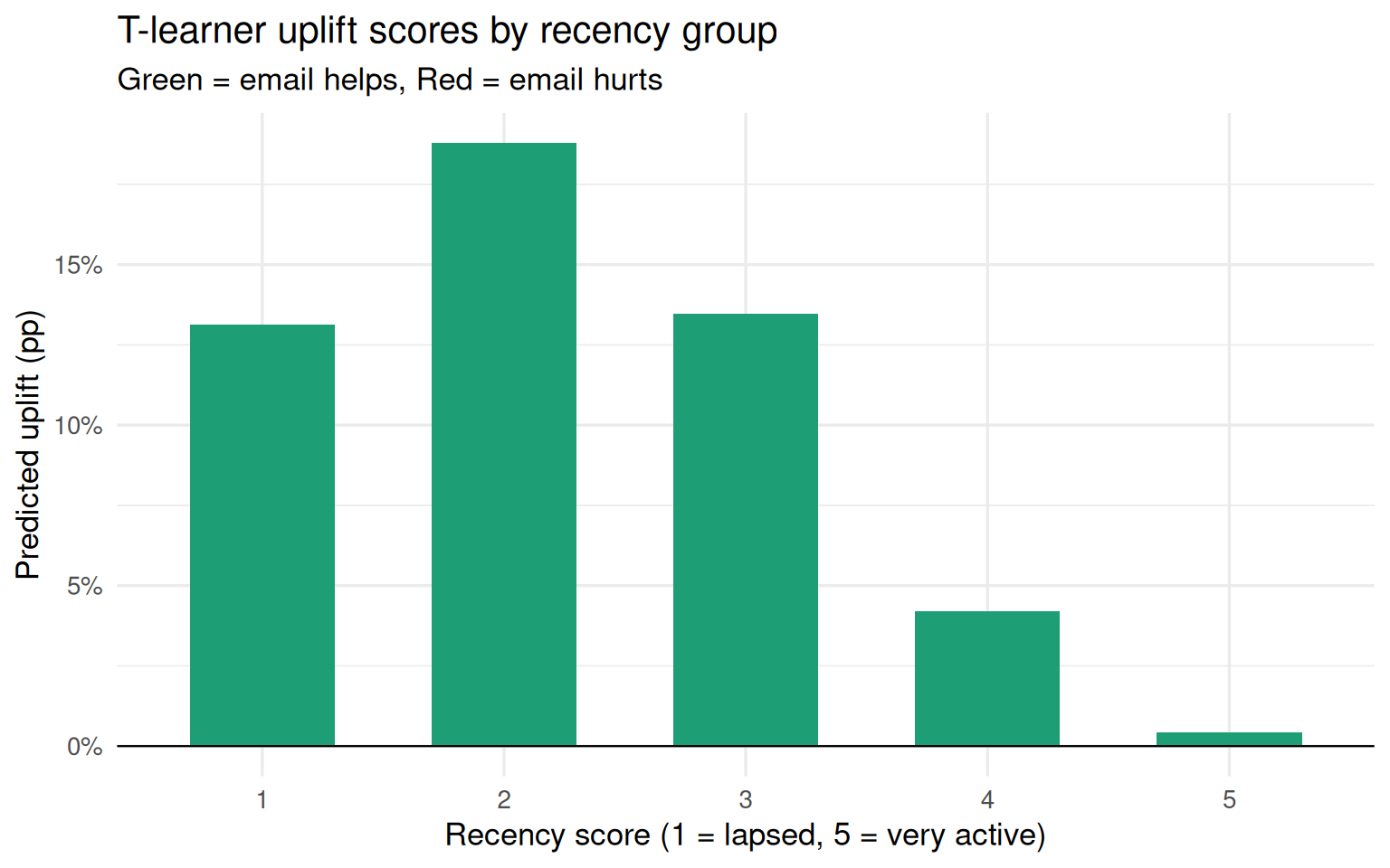
## Step 2 — The T-learner (baseline uplift model)
The simplest uplift approach trains **two separate models** — one on the treated arm, one on the control arm — and subtracts their predictions.
```{r t-learner}
# Model on treated customers only
m_treat <- glm(purchased ~ recency,
               data   = df |> filter(treatment == 1),
               family = binomial)

# Model on control customers only
m_ctrl  <- glm(purchased ~ recency,
               data   = df |> filter(treatment == 0),
               family = binomial)

# Predict for all customers under both scenarios
df <- df |>
  mutate(
    mu1_tlearner = predict(m_treat, newdata = df, type = "response"),
    mu0_tlearner = predict(m_ctrl,  newdata = df, type = "response"),
    uplift_tlearner = mu1_tlearner - mu0_tlearner
  )

# Average uplift score by recency group
df |>
  group_by(recency) |>
  summarise(
    mean_uplift = round(mean(uplift_tlearner), 3),
    .groups = "drop"
  )
```
```{r t-learner-plot}
df |>
  group_by(recency) |>
  summarise(
    uplift    = mean(uplift_tlearner),
    .groups   = "drop"
  ) |>
  ggplot(aes(x = factor(recency), y = uplift,
             fill = uplift > 0)) +
  geom_col(width = 0.6) +
  geom_hline(yintercept = 0, linewidth = 0.4) +
  scale_fill_manual(values = c("TRUE" = "#1D9E75", "FALSE" = "#E24B4A"),
                    guide = "none") +
  scale_y_continuous(labels = scales::percent_format()) +
  labs(
    title    = "T-learner uplift scores by recency group",
    subtitle = "Green = email helps, Red = email hurts",
    x        = "Recency score (1 = lapsed, 5 = very active)",
    y        = "Predicted uplift (pp)"
  ) +
  theme_minimal(base_size = 13)
```
::: callout-note
## Limitation of the T-learner
Each model is optimised to predict its own arm's outcome, **not the difference**. The subtraction compounds the noise from both models. In small samples this produces unstable uplift scores even when each individual model fits well.
:::
------------------------------------------------------------------------
## Step 3 — The Doubly Robust (DR) estimator
The DR estimator uses **both** an outcome model and a propensity score model, combined in a single correction formula. It is consistent if *either* model is correctly specified — two safety nets instead of one.
### The two models
```{r dr-step1}
# --- Propensity model: P(T=1 | X) ---
# In a perfect RCT this is always 0.5, but we estimate it anyway
# to show the principle (and because you need this for observational data)
ps_model <- glm(treatment ~ recency,
                data   = df,
                family = binomial)

p_hat <- predict(ps_model, type = "response")

# --- Outcome model: E(Y | X, T) ---
# Note: treatment IS in this model
out_model <- glm(purchased ~ recency + treatment,
                 data   = df,
                 family = binomial)

# Counterfactual predictions
df1 <- df |> mutate(treatment = 1)   # everyone treated
df0 <- df |> mutate(treatment = 0)   # everyone control

mu1 <- predict(out_model, newdata = df1, type = "response")
mu0 <- predict(out_model, newdata = df0, type = "response")
```
### The DR formula
$$
\hat{\tau}_{DR} = \frac{1}{n} \sum_{i=1}^{n} \left[
\underbrace{(\hat{\mu}_1(X_i) - \hat{\mu}_0(X_i))}_{\text{outcome model}} +
\underbrace{\frac{T_i(Y_i - \hat{\mu}_1(X_i))}{\hat{p}(X_i)}}_{\text{treated correction}} -
\underbrace{\frac{(1-T_i)(Y_i - \hat{\mu}_0(X_i))}{1 - \hat{p}(X_i)}}_{\text{control correction}}
\right]
$$
```{r dr-formula}
T <- df$treatment
Y <- df$purchased

dr_scores <- (mu1 - mu0) +
             (T * (Y - mu1)) / p_hat -
             ((1 - T) * (Y - mu0)) / (1 - p_hat)

ATE_dr <- mean(dr_scores)
cat("DR estimate of ATE =", round(ATE_dr, 3))
```
::: callout-tip
## Why the correction terms work
- **If the outcome model is perfect**: residuals `(Y - mu1)` and `(Y - mu0)` are zero everywhere, so the propensity model drops out completely.
- **If the propensity model is perfect**: the reweighting is exact and corrects for any outcome model error in expectation.
- You only fail if **both** models are wrong simultaneously.
:::
### What IPW weights are — and why they differ
A natural question is whether you could just pass `p_hat` as weights into the outcome model. No — and the direction matters:
```{r ipw-weights}
# WRONG: weights = p_hat
# This upweights people likely to be treated, amplifying selection bias

# CORRECT: Inverse Probability Weighting (IPW)
# Upweights people who were *unlikely* to end up in the arm they are in
ipw_weights <- ifelse(T == 1,
                      1 / p_hat,
                      1 / (1 - p_hat))

# IPW estimator (singly robust — only safe if propensity model is correct)
ipw_model <- lm(purchased ~ treatment,
                data    = df,
                weights = ipw_weights)

ATE_ipw <- coef(ipw_model)["treatment"]
cat("IPW estimate of ATE =", round(ATE_ipw, 3))
```
------------------------------------------------------------------------
## Method comparison
```{r comparison}
results <- tribble(
  ~Method,                ~`ATE estimate`, ~`Models needed`,     ~`Robust if outcome model wrong`, ~`Robust if propensity model wrong`,
  "Difference in means",  round(ate, 3),   "None",               "—",                              "—",
  "T-learner (2x GLM)",   round(mean(df$uplift_tlearner), 3), "2 outcome models", "No",  "—",
  "IPW",                  round(ATE_ipw, 3),"1 propensity model","Yes",                            "No",
  "Doubly Robust",        round(ATE_dr, 3), "1 outcome + 1 propensity", "Yes",                    "Yes"
)

results |>
  kable(caption = "Comparison of treatment effect estimators") |>
  kable_styling(bootstrap_options = c("striped", "hover")) |>
  row_spec(4, bold = TRUE, background = "#EAF3DE")
```
------------------------------------------------------------------------
## Targeting simulation — why uplift scores matter
If you can only email **20 customers** (40% of your list), which 20 do you pick?
```{r targeting}
set.seed(42)
# Add uplift scores from T-learner (used for targeting)
df <- df |>
  arrange(desc(uplift_tlearner)) |>
  mutate(rank = row_number())

# Strategy 1: random targeting
random_targets    <- df |> sample_n(20)

# Strategy 2: highest raw response rate (naive ML mistake)
df_response_rank  <- df |> arrange(desc(mu1_tlearner))
response_targets  <- df_response_rank |> slice_head(n = 20)

# Strategy 3: highest uplift score
uplift_targets    <- df |> slice_head(n = 20)

# Incremental purchases = purchases in targeted group - what they would have
# bought without treatment (counterfactual from control model)
incremental <- function(targets) {
  sum(targets$purchased) -
    sum(predict(m_ctrl, newdata = targets, type = "response"))
}

tibble(
  Strategy                   = c("Random", "Highest response rate", "Highest uplift score"),
  `Incremental purchases`    = round(c(
    incremental(random_targets),
    incremental(response_targets),
    incremental(uplift_targets)
  ), 1)
) |>
  kable(caption = "Incremental purchases from 20 emails — three strategies") |>
  kable_styling(bootstrap_options = c("striped", "hover"), full_width = FALSE) |>
  row_spec(3, bold = TRUE, background = "#EAF3DE")
```
------------------------------------------------------------------------
## Summary
| | Classic RCT / ATE | Uplift modelling |
|------------------------|------------------------|------------------------|
| **Question answered** | Does treatment work on average? | For whom does it work? |
| **Output** | One number | A score per individual |
| **Use case** | Policy decisions | Targeting decisions |
| **Baseline method** | Difference in means | T-learner (two GLMs) |
| **Production method** | Regression / IV | Causal forest (`grf`) |
| **Formally robust variant** | — | Doubly Robust estimator |
::: callout-important
## The key insight
The ATE is the weighted average of every individual's uplift score. Uplift modelling decomposes that average back into its parts, letting you identify persuadables (email them), sure things (skip — waste of budget), and sleeping dogs (never email — you actively hurt them).
:::
------------------------------------------------------------------------
## Further reading
- Künzel et al. (2019) — [Metalearners for estimating heterogeneous treatment effects](https://www.pnas.org/doi/10.1073/pnas.1804597116) — the X-learner paper
- Wager & Athey (2018) — [Estimation and inference of heterogeneous treatment effects using random forests](https://www.tandfonline.com/doi/full/10.1080/01621459.2017.1319839) — the causal forest paper
- Nie & Wager (2021) — [Quasi-oracle estimation of heterogeneous treatment effects](https://academic.oup.com/biomet/article/108/2/299/5911092) — the R-learner paper
- `grf` package: `install.packages("grf")` — production causal forests in R
- `uplift` package: `install.packages("uplift")` — Qini curves and uplift trees